4. Internal flows

In this section, we will consider another important practical engineering fluid dynamics problem: the flow of fluid through a duct, such as a channel or a pipe. Such problems arise in almost every engineering application, and have been studied extensively across the last 130 years. In particular, pipe flows are a particularly important application, and to this day attract considerable attention in trying to understand the physics that govern their behaviour.

We will be interested in issues such as:

• What kinds of flows arise in these settings?

• How do we estimate flowrates and flow speeds for different types of flow?

• How much ‘energy’ do we need to put into an internal flow to achieve a desired flowrate?

To do this, we first need to discuss the different flow regimes that are found in pipes and channels.

4.1. The transition to turbulence

The flow of fluid through a pipe is a classical problem that dates back to the turn of the 20th century and the original experiments of Osborne Reynolds. In 1886, Reynolds published a seminal paper that forms the basis of our understanding of pipe flows. The figure below depicts Reynolds’ experimental apparatus: a simple pipe, where the flow direction can be inferred through the injection of dye into the centreline of the pipe. It also shows the phenomena that he observed as the speed of the fluid was varied.

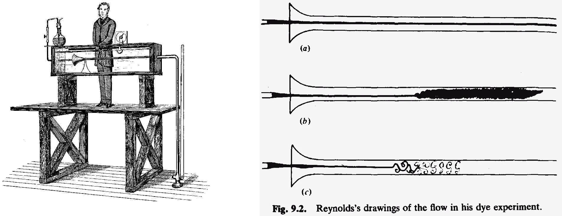
Fig. 4.1 The famous pipe flow experiments of Reynolds.

Broadly speaking, he observed the following behaviour, which you can see in the figures on the right-hand side:

• When the flow of fluid through the pipe is slow enough, the fluid flow is smooth and steady. This is called a laminar flow, since fluid particles follow smooth paths in layers. Indeed these laminar flows have mostly been the ones that we have considered thus far.

• When the speed of the fluid is increased considerably, the fluid rapidly becomes disordered and follows a more random motion, causing the dye to mix uniformly within the water. This is an example of a turbulent flow.

• There is an ‘intermediate’ regime, where the flow speed is not sufficient to have a fully turbulent flow, but not always have a laminar flow. This is the transitional regime, where the flow is a combination of turbulence and laminar flows.

These concepts are visualised in the video below. Original credit goes to the video here.

Notice that in the video above, when turbulence appears within the flow, the length of the jet arising from the end of the pipe reduces in length. This should give us some immediate conclusions: that turbulent flows offer more internal resistance and are thus ‘harder’ to push along the pipe than laminar ones.

However there are broadly more difficult questions: what is turbulence, and how do we characterise it, other than “you know it when you see it”?

4.1.1. The Reynolds number

So what governs the transitional process? In the above, we have indicated that the flow speed is the key parameter dictacting transition. However, this is not the case: if you were to repeat the experiment with the same flow speed, but changing other parameters such as pipe diameter or the type of fluid in the pipe, it would quickly become apparent that you would obtain wildly varying results.

In fact, it transpires that the flow speed is not the governing parameter here. After much experimentation, Reynolds discovered that there is a connection between:

• the diameter of the pipe \(D\), with units of length so that \([D] = \mathrm{m}\);

• average flow speed \(U\), with units \([U] = \mathrm{m}\,\mathrm{s}^{-1}\);

• the fluid’s density \(\rho\), with units \([\rho] = \mathrm{kg}\,\mathrm{m}^{-3}\);

• and its dynamic visosity \(\mu\), with units \([\mu] = \mathrm{kg}\,\mathrm{m}^{-1}\,\mathrm{s}^{-1}.\)

By observing the dimensions of these units, Reynolds realised that he could construct a parameter, which today we call the Reynolds number. This is defined as:

\[ \boxed{\mathrm{Re} = \frac{\rho UD}{\mu} = \frac{UD}{\nu}} \]

Recall that \(\nu = \rho/\mu\) is the fluid’s kinematic viscosity. If we consider the units of \(\mathrm{Re}\), we will quickly observe that

\[ [\mathrm{Re}] = \frac{[\rho][U][D]}{[\mu]} = \frac{(\mathrm{kg}\,\mathrm{m}^{-3}) \cdot (\mathrm{m}\,\mathrm{s}^{-1}) \cdot (\mathrm{m})}{( \mathrm{kg}\,\mathrm{m}^{-1}\,\mathrm{s}^{-1})} = 1\]

That is, the Reynolds number is a dimensionless parameter. Such observations are derived through a process called dimensional analysis, which is a powerful concept for the planning, presentation, and interpretation of experimental data. We will not consider this problem in this course, but you can refer to chapter 5 of the textbook by White for further information.

4.1.2. What is the Reynolds number?

So why is the Reynolds number important for the investigation of transition? Broadly:

• In a laminar flow, the fluid travels in ordered layers, with viscosity acting as a ‘checking’ frictional force between the layers, thereby keeping them all moving in the same direction.

• However, as the viscous forces are reduced, then the friction between layers will be less able to counteract the force due to the fluid’s momentum: i.e. its inertia.

• This causes small fluctuations in velocity between the laminar layers, until eventually they ‘roll up’ into a multitude of swirling vortices.

• This vortex-dominated flow is a characteristic of turbulent flows.

The difference between these states is conceptualised in the figure below.

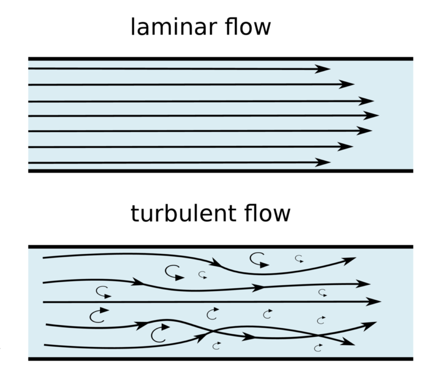
Fig. 4.2 Depiction of the difference between ordered laminar flow, and disordered turbulent flow.

The Reynolds number is a measure of this balance: it represents the ratio of inertial to viscous forces. Writing \(\mathrm{Re}\) again we can observe that the top term \(\rho U D\) is directly related to the fluid’s inertia, whereas the bottom term \(\mu\) is its viscosity. We therefore expect that:

• when viscous forces dominate, the flow is likely to be laminar;

• when inertial forces dominate, the flow is likely to be turbulent;

• and that somewhere in the middle, there is a value which tips from the flow likely being laminar to likely being turbulent: i.e. a transitional point.

4.1.3. Transition as function of Reynolds number

With the Reynolds number, we can characterise the types of flow that are found in pipe flows. By experimentation, we can show that for flow in a pipe, there is a critical Reynolds number \(\mathrm{Re}_c\), above which the flow is typically turbulent, and below which it is typically laminar.

Note

The exact value and even the definition of \(\mathrm{Re}_c\) is a topic of much debate. Recent evidence suggests that in fact \(\mathrm{Re}_c \approx 2040\), but in this course we will use a more ‘round’ number of 2000!

For pipes, we observe that \(\mathrm{Re}_c \approx 2000\), and moreover that:

• If \(\mathrm{Re} \leq 2000\), the flow is laminar.

• If \(2000 < \mathrm{Re} < 3000\) the flow is transitional.

• If \(\mathrm{Re} \geq 3000\), the flow is fully turbulent.

Example: transition in a pipe

We can readily calculate this from the Reynolds number, knowing the flow is turbulent when \(\mathrm{Re}\geq 3000\). This means that

\[ \frac{UD}{\nu} \geq 3000 \Rightarrow U \geq \frac{3000\cdot\nu}{D} = \frac{3000\cdot 1.0034\times 10^{-6} \mathrm{m}^2\,\mathrm{s}^{-1}}{5\times 10^{-2}\mathrm{m}} = 0.06\mathrm{m}\,\mathrm{s}^{-1} \]

Warning

It is important to realise that the Reynolds number can be used in a number of settings; not just for internal flows like pipes and ducts, but also for external flows such as flow over an airfoil or flat plate. In each case, the length and velocity parameters, called the characteristic length and velocity will be different and chosen on a problem-by-problem basis. For example:

• pipes use the pipe diameter and mean flow velocity through the pipe;

• flow between two plates typically uses the half-channel height and mean flow velocity;

• flow over an airfoil would use the chord length of the airfoil (roughly the distance from leading to trailing edge) and the ‘free-stream velocity’ far away from the airfoil;

and so on. In these cases, it is important to understand and use the correct parameter in your calculations. Remember also that the values we’ve given for transition are specific to pipes and do not translate to other geometries, in which transition can occur through radicially different methods.

4.2. Laminar flows

In this section we will discuss laminar flows, using as an exemplar application the flow between two plates, as we examined at the beginning of this course. We will derive some basic understanding of the velocity profile, and then move on to discuss turbulent internal flows.

4.2.1. Boundary layers

A dominant effect in internal flows is that of the boundary layer which forms due to the no-slip boundary condition. Consider the flat plate in the example below:

Fig. 4.3 A boundary layer.

The flow goes through several phases as it travels from left to right:

• Far away from the plate, the fluid travels with free-stream velocity, i.e. a uniform velocity: in this case, \(\vec{u} = U_0\hat{i}\).

• When the fluid touches the plate positioned at \(x=0\), then the fluid is brought to a halt by the no-slip boundary condition of the plate. However, the fluid above the wall still travels at the free-stream velocity.

• The shear forces acting on parallel layers of the fluid then start to slow down the layers above them.

• As the fluid travels down the length of the plate, a boundary layer develops of thickness \(\delta(x)\).

• For a laminar flow, the boundary layer observes approximately a parabolic profile so that

\[ u(x,y) \approx U\left[ 2\frac{y}{\delta} - \left(\frac{y}{\delta}\right)^2 \right] \]

• However if the flow is turbulent, the boundary layer is far more compressed and observes a power-law profile instead, so that

\[ u(x,y) \approx U\left(\frac{y}{\delta}\right)^{1/7} \]

A visual comparison between these laminar and turbulent boundary layer profiles is shown in the figure below, where we have used \(U=1\) and assumed a boundary layer thickness \(\delta(x) = 0.5\).

Fig. 4.4 Comparison of laminar and turbulent boundary layer profiles.

Boundary layers only form due to viscosity, and their presence imposes a shear stress on the wall: we denote this as the wall shear stress \(\tau_w\). Since we know from our introduction section that the wall shear stress is given by \(\tau = \mu du/dy\),

\[ \boxed{\tau_w = \mu\left.\frac{du}{dy}\right|_{y=0}} \]

Since the wall is presumably fixed in space, the fluid therefore imparts a frictional force on the wall (and vice versa) owing to the wall shear stress and, moreover, the wall shear stress will clearly be much larger in the turbulent boundary layer than the laminar one, since the gradient is far steeper! Understanding the precise mechanisms behind the transition process therefore has considerable importance.

However a detailed study of boundary layer effects is a little beyond the scope of this course, although you can refer to chapter 7 of White for more details.

4.2.2. Fully-developed internal flows

Let us first discuss a little terminology around internal flows. When the fluid enters a pipe or duct, presumably with some uniform velocity profile, then the flow will initially be two-dimensional, varying across both the length of the pipe and its radius. However, eventually, the boundary layers that form due to the no-slip condition at the wall force the fluid to increase its centreline velocity, since by conservation of mass the volumetric flowrate through any circular cross-section must be equal. This is depicted in the figure below.

Fig. 4.5 A fully-developed profile in a duct or pipe develops once it has passed a certain entrance length.

Eventually, across a distance known as the entrance length, the fluid’s velocity profile ceases to be two-dimensional, and is only one-dimensional (i.e. now a function only of radius). This is what we refer to as a fully-developed flow.

4.2.3. Velocity profile between flat plates

All the way back in the first section, we started to look at the velocity profile of a flow lying between two plates, as shown in the figure below.

Fig. 4.6 Comparison of laminar and turbulent boundary layer profiles.

Let’s now use some of our knowledge from the previous lectures to figure out what the flow profile should be analytically. Consider a small control volume of fluid with dimensions \(\delta x\), \(\delta y\) and \(\delta z\), where the \(z\)-direction travels into the page, the \(x\)-direction is horizontal and the \(y\)-direction is vertical. This is shown in the figure below:

Fig. 4.7 A small control volume

Let us now consider the conservation of momentum in the horizontal direction. Since the velocity profile is uniform in the \(y\)-direction, there is one inlet and one outlet to the control volume, and the volumetric flow rate is identical through left and right hand sides. Thus, the net flow through the CV is zero.

We then need to consider the total forces acting on the CV, which are depicted in the figure. We can begin by applying Taylor’s theorem to the left hand side surface, noting in particular that

\[ p(x+\delta x) \approx p(x) + \delta x \frac{dp}{dx}. \]

Similarly, since we know that we can write \(\tau\) as a function of velocity gradient, we know that for the top and bottom surfaces

\[ \tau(y) = \mu\frac{du}{dy} \Rightarrow \tau(y+\delta y) \approx \tau(y) + \delta y\frac{d\tau}{dy} = \mu\frac{d}{dy}\left(u + \delta y\frac{du}{dy} \right)\]

Multiplying by the appropriate surface areas of the box will yield the forces generated by the pressure and shear stress, as shown in the figure. Thus,

\[ \delta x\delta z \tau(y+\delta y) + \delta y \delta z p(x) = \delta x\delta z\tau(y) + \delta y\delta z p(x+\delta x) \]

The \(\delta z\) term immediately cancels, and we can substitute our expressions above to give

\[ \delta x \left[ \mu\frac{d}{dy}\left(u + \delta y \frac{du}{dy} \right) \right] + \delta y p(x) = \delta x \mu\frac{du}{dy}+ \delta y \left[ p(x) + \delta x \frac{dp}{dx} \right] \]

Many of these terms now cancel, leaving only the differential equation:

\[ \mu \frac{d^2 u}{dy^2} = \frac{dp}{dx}. \]

Now we can make a somewhat sneaky observation: the left-hand side of the equation involves a function only of the variable \(y\), whilst the right-hand side of the equation involves a function only of the variable \(x\). This therefore means that they must both be equal to some constant, \(c\). In other words we have that

\[ \mu\frac{d^2 u}{dy^2} = c \quad\mathrm{and}\quad \frac{dp}{dx} = c. \]

This has some really important implications. First, let’s consider pressure. This equation is telling us that the gradient of the pressure field will be constant over any given length of channel. i.e. if we start at a point \(p_1\), then after some length \(L\), the pressure \(p_2 = p_1 + c L\). We typically write this as a pressure drop \(\Delta p = p_2 - p_1\), so that

\[ c = \frac{\Delta p}{L} \]

where \(\Delta p < 0\). Now, knowing \(c\), we can solve the second equation. In particular we know that at the walls, there is a no-slip condition: therefore, \(u(\pm h) = 0\). Taking \(\mu\) over to the other side of the equation, and integrating the ODE twice, we obtain

\[ u(x) = \frac{\Delta p y^2}{2\mu L} + c_1y + c_2 \]

where \(c_1\) and \(c_2\) are two additional constants of integration: one for each time we integrated. Now we can apply our boundary conditions, which give:

\[\begin{split} \begin{align*} 0 = u(-h) &= \frac{\Delta p (-h)^2}{2\mu L} - c_1 h + c_2 \\ 0 = u(h) &= \frac{\Delta p h^2}{2\mu L} + c_1 h + c_2 \end{align*} \end{split}\]

Adding these equations gives immediately that

\[ c_2 = \frac{\Delta p h^2}{2\mu L}\]

and then subtracting the equations we see that \(c_1 = 0\). Thus,

\[ \boxed{u(y) = \frac{\Delta p}{2\mu L}\left(y^2-h^2\right) = -\frac{\Delta p h^2}{2\mu L}\left(1-\frac{y^2}{h^2} \right)} \]

We have deliberately written a minus sign in front of the equations to express that the pressure drop \(\Delta p\) is negative. If you compare this to what we obtained in the first section, you should see that the expressions are identical: we just have more information now about the flow!

This sort of parabolic flow profile is known as Poiseuille flow. We see just as before that the maximum flow velocity can be found at the centre of the channel, where \(y=0\) and so

\[ u_{\mathrm{max}} = -\frac{\Delta p h^2}{2\mu L}. \]

4.2.4. Laminar flow in a pipe

In a pipe, we have a similar problem, but our geometric coordinates are slightly different. Typically, we would express them in cylindrical coordinates so that instead of a coordinate being \((x,y,z)\) in Cartesian space, we instead identify the coordinates via \((r,\theta,z)\), where \((r,\theta)\) are the polar coordinates within a pipe’s circular cross-section and \(z\) denotes the ‘streamwise’ direction of the pipe, i.e. it’s length.

In this setting, we could follow much the same analysis: we would have a pressure drop \(\Delta z/L\) and a pipe radius of \(R\), with the velocity profile only a function of the pipe radius \(r\). This gives the Hagen-Poiseuille flow

\[ u(r) = -\frac{R^2\Delta p}{4\mu L}\left( 1 - \frac{r^2}{R^2} \right) \]

where now \(u\) denotes the streamwise velocity field.

4.3. Turbulence and turbulent flows

Turbulent pipe flows are highly important since in virtually all practical applications, some form of turbulence will arise. When we are dealing with fully turbulent pipe flows at \(\mathrm{Re}\geq 3000\), we typically consider the time-averaged quantities. This is because the flow quantities, such as the velocity, can be split into a steady average component and a time-dependent fluctuating one. Doing so reveals flow profiles that are far sharper than the laminar flow profiles, as we see below:

Fig. 4.8 Laminar vs. turbulent pipe flow profiles.

In doing so, we may ignore some time-dependent effects, however, particularly as found in the transitional regime. Although far too advanced for this course, isolated turbulent ‘pockets’ appear in these regimes that are challenging to model and quantify.

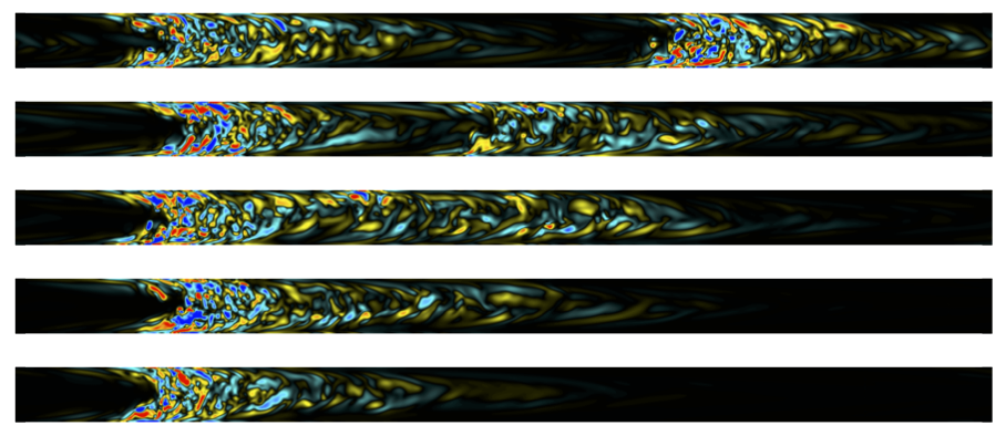
Fig. 4.9 An example of intermittent flows: an isolated pocket of turbulence (known as a ‘puff’) splits into two pockets as the flow evolves over time. These structures are inherently unsteady in time and not ameanable to the same sort of time-averaged analysis performed for fully turbulent flows.

Turbulence is a difficult concept to define, and indeed there is no formally-agreed upon definition of what constitutes a turbulent flow. However, there are characteristics of turbulence that we can define: that the motion of the flow is inherently random and domainated by vortices that span a vast range of scales. The additional energy that maintaining such vortices imposes on the flow means that turbulent flows are harder to drive (and thus require more energy to drive) than laminar ones.

In pipes the original experiments of Reynolds highlighted that pipes are extremely sensitive to the transition from laminar to turbulent flow: in other words the laminar flow profiles are inherently unstable, and at higher Reynolds numbers the flow ‘wants’ to be turbulent, rather than remain laminar. In the sections below, we’ll investigate how we can estimate the impact of turbulence on the flow physics rather than laminar flows.

4.4. Conservation of energy

Since turbulent flows are impossible to represent analytically, we need a methodology to analyse them in a more general sense. To do this, we will consider the final conservation law alongside conservation of mass and momentum: that of conservation of energy.

In this setting we have that the quantify of interest is the fluid’s total energy \(E\). We take this to be the sum of the fluid’s internal energy, its kinetic energy and potential energy (although there may be additional effects that we will not consider in the course). Then, the corresponding intensive value (i.e. energy per unit mass) is given by the quantity \(\eta\), where

\[ \eta = e + \frac{1}{2}u^2 + gz. \]

In this equation:

• \(e\) is the fluid’s internal energy and a measure of the inter-molecular forces within the fluid. This is not something we can directly measure, but we can examine how energy entering the fluid increases and decreases \(e\).

• \(u\) is the fluid velocity.

• \(z\) is the elevation of the fluid.

From our existing system formulation, we know that conservation of energy can be represented via the rate of heat transfer \(\dot{Q}\) and work done \(\dot{W}\) through the relationship

\[ \frac{dE_{\mathrm{syst}}}{dt} = \dot{Q} - \dot{W} \]

We will be reinvestigating this relationship in the thermodynamics component of the course later on. Since we need to examine this over a control volume vs. a system, we substitute this into the Reynolds transport theorem directly, so that

\[ \dot{Q} - \dot{W} = \frac{d}{dt}\int_{CV} \left(\frac{1}{2}u^2 + gz + e\right)\rho \, dV + \int_{CS} \left(\frac{1}{2}u^2 + gz + e\right)\rho\vec{u}\cdot\vec{n} \, dA\]

Now let’s start to break down the terms, starting by dwelling a little further on the two components on the right hand side as they pertain to fluid dynamics:

• In terms of heat transfer, we could start to break the \(\dot{Q}\) component down further: for example, you are likely aware that heat transferis performed via conduction, convection and radiation effects. However in this course we will not consider such effects, so that generally \(\dot{Q} = 0\), and only consider the work done component.

• The rate of work done can also be broken down into three components:

  • pressure work \(\dot{W}_p\): the work done by the pressure force;

  • viscous stresses \(\dot{W}_v\): work done by the friction forces owing to viscosity;

  • shaft work \(\dot{W}_s\): for problems that involve pumps, fans or pistons which protrude into the control volume that perform work on the system and thus ‘inject’ energy into it.

• Typically then we write the total rate of work done as \(\dot{W} = \dot{W}_p + \dot{W}_v + \dot{W}_s\).

4.4.1. The steady flow energy equation

To proceed further, we need to start making some assumptions and simplifications, as we have done in many of the previous sections. Let’s make the following assumptions:

• the flow is steady and incompressible (but not necessarily inviscid);

• the control volume has one inlet and one outlet;

• velocity, pressure and density through the inlet and outlet is uniform and normal to the inlet and outlet;

• the flow is adiabatic: i.e. there is no heat transfer.

Applying the first assumption, the time derivative disappears and we reduce the conservation of energy equation to

\[ \int_{CS} \rho\left(\frac{1}{2}u^2 + gz + e\right)\vec{u}\cdot\vec{n} \, dA = \dot{Q} - \dot{W}. \]

Considering for a moment the work done by the pressure force, we can calculate this explicitly via the standard mantra of work is force times distance: so in this case, the pressure force multiplied by the distance. If the surface has a ‘small’ area \(\delta A\) moving over a distance \(\delta x = u\delta t\) where \(u\) is the magnitude of the flow velocity, then \(W_p = p\delta A\delta x = pu\delta A \delta t\). Then summing up all of these contributions via integration, and dividing by \(\delta t\) and taking limits, we have that

\[ \dot{W}_p = \frac{dW_p}{dt} = \int_{CS} \rho\vec{u}\cdot\vec{n}\, dA. \]

We therefore typically take this into the left hand side, leaving

\[ \int_{CS} \rho\left(\frac{p}{\rho} + \frac{1}{2}u^2 + gz + e\right)\vec{u}\cdot\vec{n} \, dA = \dot{Q} - \dot{W}_v - \dot{W}_s. \]

We can then apply our assumptions 2 and 3 to obtain a far simplified relationship:

\[ \dot{m}_{\mathrm{out}} \left( \frac{p}{\rho} + \frac{1}{2}u^2 + gz + e \right)_{\mathrm{out}} - \dot{m}_{\mathrm{in}} \left(\frac{p}{\rho} + \frac{1}{2}u^2 + gz + e\right)_{\mathrm{in}} = \dot{Q} - \dot{W}, \]

where we now consider \(\dot{W}\) to just incorporate work done owing to shaft work and viscous stresses. Now, noting that by conservation of mass we must have \(\dot{m}_{\mathrm{in}} = \dot{m}_{\mathrm{out}} = \dot{m}\), and defining \(q = \dot{Q}/\dot{m}\) and \(w = \dot{W}/\dot{m}\), dividing by \(\dot{m}\) gives

\[ \left( \frac{p}{\rho} + \frac{1}{2}u^2 + gz + e \right)_{\mathrm{out}} - \left(\frac{p}{\rho} + \frac{1}{2}u^2 + gz + e\right)_{\mathrm{in}} = q - w. \]

This is called the steady flow energy equation (SFEE) and is in the form that we would typically express the first law of thermodynamics (which we’ll cover later). However in therodynamics we are typically considering compressible gases, as appear in e.g. engine cylinders. For fluids, and the kinds of problems we have been looking at thus far, it is more natural to think of incompressible fluids. Let’s therefore rework the SFEE into something that is more useful for these purposes.

Firstly we consider our fourth assumption: that the flow is adiabatic and thus there is no heat transfer so that \(q=0\). Viscosity in the fluid dissipates the kinetic energy of the fluid into heat, which we represent by the difference in internal energy between the inlet and the outlet. The equation above can therefore be written as

\[ \left( \frac{p}{\rho} + \frac{1}{2}u^2 + gz \right)_{\mathrm{out}} - \left(\frac{p}{\rho} + \frac{1}{2}u^2 + gz \right)_{\mathrm{in}} = e_{\text{in}} - e_{\text{out}} - w. \]

There are two final steps in interpreting this for fluids:

• First we rewrite the energy loss explicitly as the term \(w_L = -(e_{\text{in}} - e_{\text{out}})\).

• Secondly, viscous work is typically neglected so that the only contribution comes from shaft work – i.e. if there is a pump present in the system to do additional work in the system. In the formulation above, \(w\) denotes the work done from the system to the environment (due to its origins in thermodynamics) – but we are more interested in the opposite effect, i.e. the work performed by a pump on the fluid. We therefore write \(w_P = -w\) to reflect this.

This gives the equation

\[ \frac{p_1}{\rho} + \frac{1}{2}u_1^2 + gz_1 = \frac{p_2}{\rho} + \frac{1}{2}u_2^2 + gz_2 + w_L - w_P \]

Finally, we often express these units in height: in this way, we can interpret losses as the height that the fluid would reach if its energy were entirely converted into potential energy. \(w_L\) and \(w_P\) then translate into heights as \(w_L = gh_L\) and \(w_P = gh_P\). Substituting these into the equation above, we reach the SFEE in its final form:

\[ \boxed{\frac{p_1}{\rho g} + \frac{u_1^2}{2g} + z_1 = \frac{p_2}{\rho g} + \frac{u_2^2}{2g} + z_2 + h_L - h_P} \]

In the above, \(h_L\) is referred to as the head loss, and \(h_P\) is called the pump head. Note that it is strikingly similar to the Bernoulli equation! However since we are incorporating the head loss terms, we can apply this to viscous flows.

4.5. Head loss and friction factors

In deriving the energy equation above, we have assumed that the flow is steady, incompressible, and that there is only one inlet and outlet. These are often reasonable assumptions for pipe flows:

• in the case that the flow is turbulent, we can instead consider time-averaged values in order to apply the energy equation;

• if the inlet or outlet flow is non-uniform, it is also fairly reasonable to average the flow across the inlet of the pipe, so that the flow velocity \(U = Q/A\) where \(A\) is the area of the inlet/outlet and \(Q\) the flowrate through it.

Note

It may seem at this stage that we are being a bit cavalier in ignoring lots of effects. However remember that these equations are not designed to be exact: rather that they are used to give a reasonable estimate of the flow properties. Usually this is a good starting point, and if further analysis is required, it can always be performed either experimentally or numerically!

What does remain to be seen, however, is how we determine the energy loss term \(h_L\). Since most pipe flow problems involve turbulence in some manner, in which we cannot derive exact solutions to examine its behaviour analytically, we have to make empirical observations and derive values from experimentation. Broadly, we can categorise the losses into two categories:

• major losses are those which are due to the friction with the pipe walls;

• minor losses account for losses due to other aspects: corners, expansions/contractions, the pipe exit/entrance, valves, etc.

We will concern ourselves only mostly with major losses in this course, although we will briefly outline how they are characterised.

4.5.1. Major losses

The main loss in energy in a pipe flow is usually down to the friction force that is imposed on the fluid by the wall. There are some obvious factors that we can try to guess at what might contribute to this:

• the overall major loss is probably proportional to the kinetic energy of the fluid, since it loses part of it due to friction;

• the pipe’s length and diameter should a

• there might also be effects due to wall roughness: surfaces that have many small ‘bumps’ will likely increase drag and frictional effects;

• turbulent flows in particular have much more of their ‘bulk’ in close proximity to the wall, so we expect the frictional effects to be exacerbated vs. laminar flows.

Experimentation by a wide range of scientists has shown that the following expression (dating back to the 1850s!) gives an accurate estimate of the head loss:

\[ \boxed{h_f = f\frac{L}{D} \frac{u^2}{2g}} \]

The dimensionless parameter \(f\) which is the constant of proportionality is called the Darcy friction factor. (This shouldn’t be confused with the Fanning friction factor, which is conceptually the same but differs by a factor of 4). The friction factor is generally a function of three things:

• the Reynolds number \(\mathrm{Re}\);

• the relative wall roughness \(\epsilon/d\);

• and the shape of the duct (in this case we ignore this since we are only interested in pipes).

4.5.1.1. Smooth laminar flows

In the case that the flow is laminar and the pipe is smooth, we can actually derive the friction factor analytically, since we have a formula for the flow profile \(u(r)\). Consider a section of pipe with fully-developed laminar flow. Flow enters at the section 1 and exits at section 2, where the pipe is also angled at \(\phi\) to the horizontal direction.

Fig. 4.10 Control volume of a steady, fully-developed laminar flow between two sections in an inclined pipe.

Consider a control volume that is simply the whole pipe section. The flow is fully developed so the velocity at the inflow and outflow are equal to some value \(U\). Our energy equation therefore tells us that

\[ \frac{p_1}{\rho g} + \frac{U^2}{2g} + z_1 = \frac{p_2}{\rho g} + \frac{U^2}{2g} + z_2 + h_f \Rightarrow h_f = (z_1 - z_2) + \left(\frac{p_1}{\rho g} - \frac{p_2}{\rho g} \right) = \Delta z + \frac{\Delta p}{\rho g}. \]

Now, we can apply continuity of momentum with one inlet and one outlet in the \(x\)-direction, where \(x\) is aligned with the centreline of the pipe. The forces on the control volume are:

• pressure: the force on section 1 is \(p_1 A\), and the force on section 2 is \(-p_2 A\), giving a net force of \(\Delta p A\).

• gravity: calculated as \(F_g = \rho g AL\sin\phi\);

• viscosity: this is calculated using the wall shear stress \(\tau_w\), where the total surface area of the cylinder is \(2\pi R L\) and thus the overall force is \(-\tau_w \pi D L\), where the force is negative since it acts in the opposing direction to the fluid that flows from point 1 to 2 in the \(x\)-direction.

The conservation of momentum tells us that the sum of these forces must be equal to the overall change in momentum, i.e.

\[ \Delta p \pi R^2 + \rho g\pi R^2 L\sin\phi - 2\tau_w \pi RL = \dot{m}(U - U) = 0. \]

Dividing this equation by \(R^2 \rho g \pi\), and noting that \(\Delta z = \sin\phi\) from the geometry of the figure, we can simplify this to

\[ \frac{\Delta p}{\rho g} + \Delta z = \frac{2L\tau_w}{R\rho g} = \frac{4\tau_w}{\rho g}\frac{L}{D} \]

The left hand side is identical to the expression we derived above using the energy equation, so

\[ h_f = \frac{4\tau_w}{\rho g}\frac{L}{D}. \]

Note

Note that the head loss is proportional to wall shear stress, regardless of whether the pipe is horizontal or tilted.

We can now actually do something with this! We know that the flow velocity is given by the function

\[ u(r) = u_{\mathrm{max}} \left(1 - \frac{r^2}{R^2} \right) \]

Moreover, we know that the mean velocity of the pipe \(U\) and the maximum centreline velocity are related as \(u_{\mathrm{max}} = 2U\), since the average velocity is calculated via the integral over the circular cross-section:

\[\begin{split} \begin{align*} U = \frac{1}{A} \int_0^{2\pi} \int_0^R u(r) r\, dr\, d\theta &= \frac{2\pi u_{\mathrm{max}}}{\pi R^2} \int_0^{R} \left( r - \frac{r^3}{R^2} \right) dr \\ &= \frac{2 u_{\mathrm{max}}}{R^2} \left[ \frac{r^2}{2} - \frac{r^4}{4} \right]_0^R \\ &= \frac{2 u_{\mathrm{max}}}{R^2} \cdot \frac{R^2}{4} = \frac{1}{2}u_{\mathrm{max}}. \end{align*} \end{split}\]

Note

The additional \(r\) in the first integrand comes from the curvilinear integral over the circle’s polar coordinates.

Since we have the flow profile, we can compute the wall shear stress analytically. Noting that our original definition of wall shear stress uses the distance from the wall \(y\), we have to now modify the direction slightly to account for \(r\) orignating from the centre of the pipe, which is in an opposing direction. Thus, we have

\[ \tau_w = \mu\left.\frac{du}{dy}\right|_{y=0} = -\mu\left.\frac{du}{dr}\right|_{r=R} = \mu \frac{2u_{\mathrm{max}}}{R} = \frac{4U\mu}{R} \]

Therefore,

\[ h_f = \frac{4L}{\rho g D} \cdot \frac{4U\mu}{R^2} = \frac{32LU\mu}{\rho g D^2}. \]

Finally then, we have that the friction factor is given by

\[ f = h_f \cdot \frac{2Dg}{LU^2} = \frac{32\mu LU}{\rho g D^2} \cdot \frac{2Dg}{LU^2} = 64 \cdot \frac{\mu}{\rho U D} \]

or in other words,

\[ \boxed{f_{\mathrm{lam}} = \frac{64}{\mathrm{Re}}}. \]

Several rearrangements of the equations above are possible to calculate head losses in laminar pipes: the most useful are in terms of either the flowrate or flow velocity:

\[ \boxed{h_f = \frac{32\mu LU}{\rho g D^2} = \frac{128\mu LQ}{\pi\rho g D^4}} \]

4.5.1.2. Turbulence and wall roughness

In order to understand how friction factors vary for turbulent flows and wall roughness, we must first define what we mean by roughness? Typically, we express this in two ways.

• The absolute roughness \(\epsilon\) is measured in units of length, and typically in \(\mathrm{mm}\). This is a measurement of the mean deviation between a smooth wall and the irregularities in the surface. We take the mean since at small scales, the roughness will be an inherently ‘random’ function of position along the wall which fluctuates around some mean value.

• The relative roughness \(\epsilon/d\) is a dimensionless ratio that represents the relative roughness accounting for the diameter of the pipe. This is typically the most useful measurement for us, since roughness effects will be far less pronounced in larger pipes than smaller.

By running experiments at varying Reynolds numbers and relative roughnesses, we can make some observations in their behaviour, as shown in the figure below.

Fig. 4.11 Experimental data performed at various Reynolds numbers for a selection of pipes with differing roughness factors.

These experiments led the fluid dynamicist Colebrook in 1939 to observe the empirical relationship

\[ \boxed{\frac{1}{\sqrt{f}} = -2\log_{10}\left( \frac{\epsilon / d}{3.7} + \frac{2.51}{\mathrm{Re}\sqrt{f}} \right)} \]

This is a somewhat awkward expression, since it is transcendental: that is, if we are interested in computing \(f\) directly, there is no way to rearrange the expression in terms of \(f\)! Other examples you might have seen before that demonstrate this are trying to solve equations such as \(x + \sin x = 0\).

However this does not mean that there is not a solution. We can compute solutions numerically on computer, and then visualise them in a graph.

4.5.1.3. Moody charts

A Moody chart, so named after its creator, is such a way to visualise the relationship between friction factor, Reynolds number and pipe roughness. A Moody chart for water is shown in the figure below.

Fig. 4.12 Moody chart for pipe friction with both smooth and rough walls.

The way to use a Moody chart is to:

• identify a relative roughness that is close to the value you are looking for – if you are in-between, you’ll need to interpolate between curves;

• read the Reynolds number on the \(x\)-axis and draw up to the line for that value of roughness;

• read off the friction factor on the left hand side.

Warning

Note that both \(x\)- and \(y\)-axes are in logarithmic scale, so it is important to be mindful of this when reading values!

4.5.1.4. Typical values of wall roughness

We can collate experimentally the absolute wall roughnesses for a range of materials. Table 6.1 in White is partially reproduced here for your reference.

Material	Type	Wall roughness \(\epsilon\,[\mathrm{mm}]\)
Steel	Sheet metal	0.05
	Stainless	0.002
	Rusted	2.0
Iron	Cast	0.26
	Wrought	0.046
Glass	-	Smooth
Concrete	Smoothed	0.04
	Rough	2.0
Rubber	Smoothed	0.01
Wood	Stave	0.5

4.5.1.5. An example

Example:

Oil, with \(\rho = 900\,\mathrm{kg}\,\mathrm{m}^{-3}\) and \(\nu = 0.00001\,\mathrm{m}^2\,\mathrm{s}^{-1}\), flows at \(0.2\,\mathrm{m}^3\,\mathrm{s}^{-1}\) through \(500 \mathrm{mm}\) of \(200\,\mathrm{mm}\) diameter cast iron pipe. Determine (a) the head loss and (b) the pressure drop if the pipe slopes down at \(10^\circ\) in the flow direction.

Firstly, let’s compute the velocity from the known flowrate. We have that

\[ V = \frac{Q}{\pi R^2} = \frac{0.2}{\pi 0.1} = \frac{2}{\pi} \approx 6.4\,\mathrm{m}\,\mathrm{s}^{-1} \]

Then we can compute the Reynolds number as

\[ \mathrm{Re} = \frac{UD}{\nu} = \frac{6.4\cdot 0.2}{0.00001} = 128000. \]

Reading the table above we can compute that \(\epsilon = 0.26\,\mathrm{mm}\) for cast iron pipe. So, the relative roughness is given by

\[ \frac{\epsilon}{D} = \frac{0.26}{200} = 0.0013 \]

Now if we read the Moody chart, by starting at the right-hand side for relative roughness, we can read off a value of around \(f\approx 0.0225\). Then the head loss is given as

\[ h_f = f\frac{L}{D}\frac{U^2}{2g} = 0.0225 \frac{500}{0.2}\cdot\frac{6.4^2}{2\cdot 9.81} = 117\,\mathrm{m} \]

Finally, from our energy equation, we have that

\[ h_f = \frac{\Delta p}{\rho g} + z_1 - z_2 = \frac{\Delta p}{\rho g} + L\sin 10^\circ, \]

or if we rearrange for the pressure drop, this gives

\[ \Delta p = [h_f - 500\cdot\sin 10^\circ] \approx 265\,\mathrm{kPa}. \]

4.5.2. Minor losses

As we noted before the extended discussion on major losses, there do exist also minor losses that account for aspects like bends in the pipe, expansions/contractions, valves, and other such obstructions. Such losses are difficult to account for analytically: typically, they might introduce additional turbulence into the flow that is essentially impossible to quantify without experimentation or simulation.

Since these aspects are challenging to account for in terms of the flow patterns they generate, we typically represent the minor loss as a ratio of the head loss through the device to the velocity head of the piping system. That is, we express this as

\[ h_l = K\frac{U^2}{2g} \]

The coefficient \(k\) is something that has to be defined for the particular obstacle. For example, a manufacturer of a valve might supply a chart showing the value of \(K\) that is suitable depending on the fraction of flow allowed through the valve. We can also account for things like corners in this manner. Consult the textbook by White for more information on specific values for \(K\).

Warning

Although ‘minor’ may indicate that these losses are trivial in comparison to major losses, this isn’t necessarily the case! Minor losses, particularly in complex pipes that have many bends and fittings, can often far outweight major losses.

4.6. Summary

In this section we have covered many aspects of internal flows:

• the Reynolds number and how it affects laminar vs. turbulent flows;

• conservation of energy and the steady energy equation;

• major losses in pipes;

• calculating friction factors and accounting for wall roughness.

In the final section of this fluids course, we will consider the alternative formulation of fluid dynamics problems in differential form by exploring the Navier-Stokes equations.

Further reading

For further reading, consult chapter 6 of White. In particular:

• section 6.1 for an overview of Reynolds numbers;

• section 6.3 for head losses and the friction factor;

• section 6.4 for fully-developed laminar flows;

• section 6.7 for examples of applying these equations to pipe flow problems;

• and section 6.9 for minor losses.